I’m working on a compiler, and testing it has been interesting, so that’s what we’re going to talk about. My take-aways are that:

1. The best / most efficient way to test my compiler is with end-to-end system testing (see the section on System Testing & Why it’s a good choice)
2. Figuring out which inputs to test is the most interesting part (see the section on Testing Modes)

Big Picture

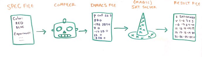
I’m working on a compiler that helps solve the following problem: you’ve got N objects and you want to find some ordering of them, but you’ve got some constraints about the ordering that you need to satisfy.

The way we’re going to solve this problem is by writing down these constraints in a way that a SAT solver can understand, and having the solver do the heavy lifting to finding an ordering that satisfies the constraints.

I’m writing a compiler because the SAT solver input format isn’t feasible to write by hand, but it’s not too painful to generate. So my compiler translates a nice human readable representation of the constraints down to this DIMACS SAT input format. 😟 -> 🤖 -> 😎

I’ll talk more about the nitty gritty of this compiler in different post because what I really want to focus on about now is how to test this compiler.

The tl;dr of how I test my compiler is I have a program that generates a bunch of inputs to the compiler pipeline, and a bash script that runs the pipeline and validates that the outputs make sense given the inputs.

In the next section I’ll briefly explain what my compiler does, but if you just want to read about system testing compilers you can skip to the following section.

What my compiler does

I’m going to give you a 30,000 foot overview of the compilation pipeline, because it’ll ground the testing discussion and also because it’s interesting.

Inputs: Objects & Constraints

Objects

Like I said above, my compiler translates constraints about sequences of “objects”. An object is just a record with fields.

Let’s say the objects we want to order have a shape circle or square and a color red or blue. Let’s say we’ve got N of each of these objects. This means we’ve got a set with N instances of each of

• red square
• red circle
• blue square
• blue circle

and what we want is to put these objects some order, subject to some constraints. That’s what I call a “fully crossed” set of size N (which you’ll see in the example input file below).

Examples of constraints

Here are examples of some of the ways we might want to constrain the ordering:

• No more than 2 red objects in a row
• Out of every 7 consecutive objects, we must have at least 1 blue square
• As many red objects followed by blue objects as red followed by red
• The first object must be a red circle
• Every 5th object must be either a red circle or a blue square

This isn’t a comprehensive list, but it should lend some intuition about the types of constraints we’re dealing with.

One thing to notice is that constraints take arguments. For instance, “no more than k values in a row” takes the arguments k and value, which are the numeric limit (ie 2) and the value that we want to limit the repetition of (ie red).

Putting them together: Specification File format

The specification file format is a format I made up. Here’s an example of how one might look:

Features:
  Color:
      Red
      Blue
  Shape:
      Circle
      Square

Experiment: 4 x Fully_Cross( Color, Shape )   //like the example above in 'Objects'

Constraints:
    < 3 (Color:Red) Consecutively

Outputs: DIMAC

The format I’m compiling to is something called DIMACS CNF. There’s an example below, but it basically looks like a big list-of-list of numbers. This isn’t very human readable and a bit finicky to generate, which is exactly why I want to be very careful about testing my compiler.

p cnf 367 1992
368 0
369 -366 0
-369 366 0
370 -367 0
-370 367 0
375 -357 0
-375 357 0
-384 0
-386 -375 -383 384 0
-386 -375 383 -384 0
-386 375 -383 -384 0
-386 375 383 384 0
386 -375 -383 -384 0
386 -375 383 384 0
386 375 -383 384 0
386 375 383 -384 0
-385 375 383 0
-385 375 384 0
-385 383 384 0

Like that for thousands of lines. And that’s for a simple constraint! Complicated combinations of constraints can produce files that are hundreds of thousands of lines long.

Compiler Pipeline

Here’s the whole pipeline.

1. Given a specification file, my compiler will generate a DIMACS file.
2. I feed the generated DIMACS file into a SAT solver.
3. The SAT solver outputs a result file that is also just a list of numbers.
4. I can then post-process this result file to see the ordering that the solver found.

System Testing & Why it’s a good choice

When I say “system testing” I mean that I’m testing the complete system instead of testing modular functions, the way you would with unit testing. This means my tests will create files that go into the beginning of the entire pipeline (specification files, which consist of objects & constraints) and validate the final output file produced by the SAT solver at the end of the pipeline.

Why not Unit Testing?

If I was unit testing my compiler, I would take each function and write tests that validated the output of that function for various inputs. The functions in my compiler represent different increasingly complicated constraints. Every function returns a valid CNF boolean formula. These CNF formulas are:

• long
• not very comfortable to think about, and
• not fun to write by hand,

which makes these functions not conducive to unit testing. If I was unit testing them, I would need to work many examples by hand, and my results would probably be error-prone and wouldn’t cover the test space very well.

You might be thinking, but you could do both! True, but there’s a great adage about testing: you should keep testing until your fear turns to boredom. I’m vigilant in my testing because I’m distrustful of my compiler being buggy, but I’m confident that my system tests cover the same ground as unit tests would, but more efficiently.

Advantages of System Testing

What I really want to know is that I’m communicating with the SAT solver correctly. The input to the SAT solver is literally the specification I’m trying to match, and this is exactly what system testing is validating.

Another advantage is that once I set up validation for each different kind of constraint, I have a framework that can test any combination of constraints for free. That’s neat because you could even use that in production- when you have a “real” ordering you want to generate, you can automatically validate that the ordering you get out of the pipeline actually satisfies the constraints you put in.

The Testing Pipeline

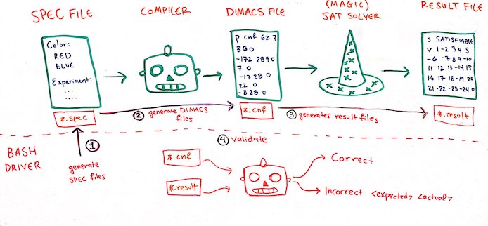
Okay, so what I want to do is test that my compiler produces the correct DIMACS files for each kind of constraint.

1. For a given constraint, generate a specification file. Lots of discussion about this in the following section.
2. Put the specification file through the compiler, producing a DIMACS file.
3. Push the DIMACS file through the SAT solver, producing a result file.
4. The compiler slurps in the specification file & the result file, and validates that the resulting sequence does actually satisfy the constraints in the specification file.

Below I’ll talk about the interesting different ways we can generate specification files, and then talk about some details from my implementation.

Testing Modes

There are three testing modes: exhaustive, random and on-demand. The ONLY difference between these testing modes is how the specification files (which are the input to the pipeline) are generated.

Exhaustive Tests

I test individual constraints “exhaustively”. These are as close as I come to unit testing.

Exhaustively in quotes means: exhaustively, with some caveats. Recall that constraints take arguments, and when I say “exhaustive” I mean that we’ll exhaustively generate a specification file for every “important” argument to the constraint we’re testing. Recall also that these specification files define which objects the constraints apply to; for testing I have 4 predefined object sets that I can choose from.

First I select a constraint (like “fewer than k out of every n”) and an object set, and then my program fills in values to all the other arguments to that constraint. The arguments to “fewer than k out of every n” are the value the constraint is applied to and the values of k and n. The value n is determined from the number of objects in the object set, and value is always red. It shouldn’t matter what specific value I choose for testing, and red is present in every object set. The program will try every possible meaningful value of the remaining argument k, so I’ll generate a specification file with every value from 0 to n.

If you want to see what these object sets look like, I’ve included descriptions of them in the Appendix. The take-away is they include sets of objects that reflect how the compiler works internally, so if one set of objects passes but another fails, that can be used to disprove certain classes of bugs. The final and most complicated object set should be representative of how the compiler treats arbitrarily complicated object sets.

An example of how I would call these tests looks like:

./test exhaustive fewer-than-k-out-of-every-n simple-object

The benefits of exhaustive tests is they thoroughly test constraints for at least small and relatively simple object sets.

The drawbacks are that it’s not feasible to use these tests for large object sets, and they don’t test combinations of constraints. I also don’t test different values except red. This seems sketchy, but it blows up the search space for something that’s treated very symmetrically inside the compiler. The random tests below do use different values, so I feel comfortable with that compromise. (knock on wood)

Random Tests

Random testing tests combinations of constraints. This is a really simple fuzzer! It’s like putting a firehose of random inputs into the pipeline and seeing if things still come out the way we expected them on the other end.

The way my random testing works is we’ve got all the constraints in one hat, and all of the possible argument values in another hat. We’ll draw constraints and matching arguments at random and generate constraint files from them. The number of constraints we try combining is chosen at random between 1 and 4. There are a few hyper-parameters:

1. The number of times to re-draw random constraints
2. Once we’ve selected the constraints, the number of times to re-draw random arguments to those constraints.

Some constraints/argument combos don’t work together: for instance, you can’t demand that you have fewer than 2 red values in a row, and also greater than 2 red values in a row. However, negative testing is also valuable so I hold on to these impossible specification files. The file the SAT solver returns should complain that it couldn’t find a valid ordering, and when we validate these files there’s some logic to compute whether or not we expect a negative result.

Like the exhaustive tests, we choose from the testing object sets. Unlike the exhaustive tests, we choose a value at random to be the value argument to the constraints.

export constraint_draws = 10
export argument_draws = 100
./test random constraint_draws argument_draws simple-object

The benefits of random testing is that it’s a way to test lots of more complicated situations. The drawbacks are that these random tests don’t cover the sample space very thoroughly. They just cover the test space randomly, but that might not be representative of realistic constraints.

Another drawback is I don’t fuzz over possible objects. This is because I don’t think this is a likely source of bugs, and so it’s not worth the extra effort. (Watch me jinx it)

On-Demand Tests

“On demand” testing is for when you have a particular specification file that you want to validate. This option just short-circuits the specification file generation part of the testing framework.

An example of how I would call these tests looks like:

./test on-demand specification-file simple-object

Implementation details

My tests are orchestrated by a bash script. This script calls my compiler with various command line arguments which runs all the compiler-related parts of the pipeline- like generating & parsing files- and also feeds appropriate files through the SAT solver. (See the diagram above under “testing pipeline”). Each step generates files in a tests directory, and at the end of every run the script clears out the testing directory. Everything runs on command line arguments.

Generating Specification Files

This is exactly what we discussed above about the “testing modes”. Each mode specifies how to generate specification files, and the mode and the corresponding hyper-parameters are specified with command line flags.

Each file is named a consecutive number, so files end up looking like 0.spec.

Generating DIMACS files

The bash script tells the compiler to generate DIMACS files for every file in the testing directory. The compiler parses each specification file and internally calls the corresponding functions with the corresponding arguments. It produces n DIMACS files, which are named with the same number as the specification file they were generated with.

There are now 2n files in the directory of the form 0.cnf and 0.spec.

Running the SAT solver

The bash script then grabs every *.cnf file in the testing directory, and runs it through the SAT solver. It pipes the output to a *.result file with the corresponding number.

There are now 3n files in the directory of the form 0.result, 0.cnf and 0.spec.

Validating Generated Result files

The bash script then tells the compiler to validate every *.result file in the directory. To do this, the compiler reads in every *.result and also every *.spec file. We then use the same spec parser that we used to generate the DIMACS files we extract the constraint and the arguments to the constraint, as well as the set of objects. The compiler uses this to interpret & validate the *.result file.

The result of the validation is printed to stdout:

• If the test case passes, then the compiler is silent (by default), or emits Correct (if the verbose flag was passed)
• If the test case fails, then:
  • If it fails because of a parse error, it emits ParseError
  • If it fails because the SAT solver didn’t find an ordering, it emits UnsatisfiableError
  • If it fails because the sequence didn’t satisfy the constraints, it emits WrongResult <expected> <actual>

If the test case fails, the compiler writes the result and spec files to a failedTests directory.

The bash script then scrapes the tests directory clean.

Appendix

Details that I didn’t think were interesting enough to include above.

The Actual Tests

I’ve talked about the kinds of tests I can run, here is what my testing wrapper actually runs:

• Exhaustive Tests
  • For every constraint
    • For every object test set
• Random Tests
  • 50 constraint draws
    • 50 argument draws

With those parameters, the random tests test 50*50 = 2,500 random configurations. I can run the random tests multiple times to increase their test coverage, because every time is a new random check in the search space. Because each run generates (and then deletes) 7,500 files, I think that’s a good upper limit for the size of a single iteration of search. There’s also an “over-the-weekend” mode where I’ll run the random tests 100 times (or until I decide to kill the script) for 250,000 random configurations.

Any test that fails is copied into the failedTests directory, and I can rerun that test using the “on-demand” testing mode.

Object Sets for Testing

I have four object sets available for testing. Each of these is “fully-crossed” as defined in the ‘What My Compiler Does’ section, and each one has 20 instances of each possible object.

1. The simplest possible objects: Each has a single field “color” with 2 values. There are 2*20 = 40 objects in this set.
   • red
   • blue
2. Objects with more values: Each has a single field “color” with 3 values. Objects with 3 fields are treated differently than objects with 2 fields internally, so this object set is meaningfully different than the first one. There are 3*20 = 60 objects in this set.
   • red
   • blue
   • green
3. Objects with more fields: Each has two fields “color” and “shape” each with two values. Similarly, objects with more than 1 field are treated differently internally, so this object set is also meaningfully different than the first two. There are 4*20 = 80 objects in this set.
   • red square
   • blue square
   • red circle
   • blue circle
4. A complicated object set: Each has 3 fields “color”, “shape”, “saturation”, each with 2 or 3 values: 20*12 = 240 objects in this set.
   • dark red circle
   • light red circle
   • dark red square
   • light red square
   • dark red triangle
   • light red triangle
   • dark blue circle
   • light blue circle
   • dark blue square
   • light blue square
   • dark blue triangle
   • light blue triangle